Eric Weeks - personal pages - pictures Cellular Automata Phase Diagrams

weeks@physics.emory.edu

NOTE: The large phase diagram picture is related to the "dripping rail" Cellular Automata; click on it to see some variations on that rule. (The large one a little further down the page, not one of these top four.)

These pictures relate to phase diagrams which I generated a long time ago, and I no longer know exactly which are which.

When I was at the 1995 Complex Systems Summer school at the Santa Fe Institute, I worked on cellular automata with real numbers describing the state of each cell. I wrote a program that would generate CA's with the restriction that the state of each cell was a real number between 0 and 1. The update rule was restricted to:

new x_{n} = A x_{n-1} + B x_{n} + C x_{n+1} + D mod 1 .

I quickly generated a large number of CA runs starting from a random initial state. Many of them looked "boring" -- the final state would be a uniform gray color, or worse, a uniform black color (black = 0). But some looked very interesting.

I then worked on the meta-level question, what values of the parameters A, B, C, and D would give me "interesting" CA rules. I have a very nice four-dimensional phase space plot but unfortunately the limits of HTML and most conventional monitors prevent me from showing you this four-dimensional picture. :-) Actually, I added the further restriction A = C, to simplify matters further.

Various cuts through the four-dimensional phase space are shown below. The random appearance of parts of the plot is due to the random initial conditions.

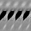
For this first plot, D ranges from -2 to 2 (horizonal axis), A = C and range from -2 to 2 (vertical axis; -2 at top of the plot), and B=0.2 is fixed. In this plot, black is zero, white is 1/2. Given that the arithmetic of the rule is done mod 1, the plot is periodic in D.

Click here, or on the picture, to see some CA patterns taken from various places in this phase diagram above.

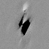
Here is another phase diagram. In this case, A = C = 0.2 is fixed, D ranges from -2 to 2 (horizonal axis), and B ranges from -2 to 2 (vertical axis; -2 at top). Again, black is zero, white is 1/2, and the plot is periodic in D.

Click here to see a large version of this phase diagram.

For this last phase diagram, D = 0.2 is fixed. A = C is plotted on the horizontal axis, and ranges from -2 to 2. B is plotted on the vertical axis, and ranged from -2 to 2 (-2 is at the top of the plot). Black is zero, white is 1/2, and this plot isn't periodic.

Click here to see a large version of this phase diagram.

Links...

• Questions? Comments? Send me email; email address below.
• Other pictures I've made - quasicrystals, fractals, cellular automata, other things.
• Software I've written -- some functional, some fun
  
• Various simple algorithms for making simple pictures
  
• Research I do
  
• Graphics techniques (some used to make this picture)
  

• Click here for information about the software I use to make cellular automata.