Using GameBug

This introduction assumes that you already know the basics of game theory and want to use GameBug to work with payoff matrices. If you do not yet know game theory, go through one of our web tutorials along with GameBug and this manual. (Download a pdf copy of this manual here.)

Getting Started

To start with an empty game, double-click GameBug.exe. The Examples folder contains several pre-defined games. To open one, double-click its document icon (shown here). GameBug documents have a .gbg extension.    

Configuring a Game

When you open GameBug, it shows a window with an empty 2×2 payoff matrix:

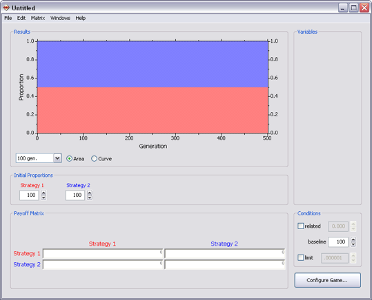
If all you need is a 2×2 payoff matrix containing only numbers, just type those numbers into the payoff matrix and the results graph will automatically update to show how each strategy fares. For anything more complex, click the Configure Game button at the lower right corner of the window or type ctrl-G to select it from the Matrix menu. It will show the following window:

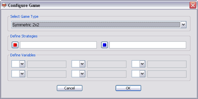
The first popup menu sets the game type (symmetric 2×2 to 6×6 or asymmetric 2×2 or 3×3). Next, you can assign a name and color to each strategy. The names are used to label the payoff matrix and colors are used in the results graph. Finally, you can define up to six variables for use in the payoff matrix. Variables are single letters and may be lower- or uppercase (a and A are different variables). You may also give a descriptive name to each variable. Click OK to accept the changes and return to the main window or Cancel to leave the game unchanged.

Payoff Matrix

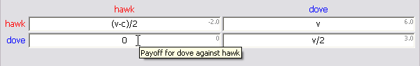
The payoff matrix is defined at the bottom of the window. For a symmetric game, each cell contains the payoff for that row against that column. When the mouse is held over a cell, a yellow tooltip shows which payoff that cell defines:

An asymmetric game requires two matrices, one for each role. Each matrix is labeled with its role and contains the payoffs for that role against the other role:

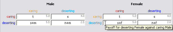
The upper-right corner of each payoff shows the numerical value of the payoff given current variable values. When you change variable values, these numbers are recalculated so that you can always see what the payoffs actually are.

A payoff may contain any algebraic expression using variables, numbers, parentheses and brackets, arithmetic operators (+, −, /, ^), the constants π and e, and the functions ln(a) (natural log), max(a,b) (maximum of a and b), min(a,b) (minimum of a and b), and fct(a) (factorial of a). To enter π or e, use the Matrix menu. For roots, use fractional exponents (√a = a^0.5). All of the following are valid payoffs (assuming variables a, b, and c are defined): ab/c, 2a, 2ln(b), e^-b, min(a,2b), and 2 + 3 a. You may put spaces between variables for clarity, but do not put space between a function name and parenthesis (ln (a) would be treated as l × n × a). No special operator is needed for multiplication: 2 × a is just 2a.

If there is an error in a formula, the background of that payoff cell turns pink and the payoff is treated as zero in fitness calculations.

Initial Proportions

By default, all strategies start in equal proportions and evolve from there. To change the initial proportions, type a number in a proportion box or use the up-down arrows to the right of the box. These proportions are relative. Thus in a 3×3 game, proportions of 100, 50, and 50 are 50%, 25%, and 25% respectively. To see the percentage, hold the mouse over a proportion and the percentage will appear in a yellow tooltip box.

Variables

If you defined variables when configuring the game, they will appear in a column to the right of the results graph. To change the value of a variable, type a number in the box, use the up-down arrows next to the box, or click the box and roll the mouse wheel. When a variable value changes, the payoff matrix is recalculated and the results plot is updated.

Conditions

Below the column of variables is a set of special conditions that can be changed:
Relatedness. To test the effect of genetic relatedness, check this box and specify the relatedness of the players (0 to 1). If the box is not checked, the value is ignored. (When relatedness is used, payoffs are calculated by neighbor-modulated fitness in symmetric games and by Hamiltonian inclusive fitness in asymmetric games.)
Baseline. This is the fitness that each player starts with in each generation. It increases or decreases by the payoff received when the game is played. Making baseline fitness higher slows change over generations but does not alter the outcome.
Limit. GameBug normally treats a population as infinite. If the limit box is checked, all proportions are rounded to multiples of the specified limit. This mimics a limited population (e.g. a limit of 0.0001 implies a population of 10000).

Results

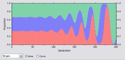
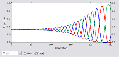
The graph shows how the proportion of each strategy in the population changes over time. You can increase the number of generations shown by changing the number of generations per tick mark (popup menu below the graph) or by expanding the window. By default, GameBug shows proportions by shading the graph area, which makes it easy to see which strategy dominates. You can instead show proportions as curves ranging from 0 to 1 by selecting the Curve button below the graph.

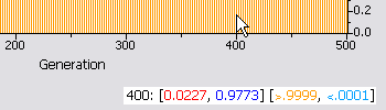
When the mouse is held over the graph, text appears below the graph showing the generation that the mouse is over and the numerical proportion of each strategy at that generation. Move the mouse along the plot to see how proportions change with time. This example shows the results of a 2×2 asymmetric game at generation 400. The proportions for each role are grouped in brackets and color-coded by strategy:

When you enlarge the GameBug window, the graph area grows, showing more generations and giving more detail of proportions.

Mutations

You can introduce a “mutation” into the game with a right-click (control-click) on the results graph. If a strategy is absent at the generation where you clicked, you can add it at a low level to see if it increases. If a strategy is present, you can remove it to see how the other strategies react. The mutation technique can be used to test whether a novel strategy can invade a stable game: Start with the proportion of the novel strategy set to zero and then introduce it as a mutation after the other strategies have come to equilibrium.

Notes

Text notes can be stored with the game for future reference. Show or hide the Notes window by typing ctrl-T or selecting it from the Windows menu.

Printing and Saving Data

When you have created a new game or found a combination of variables that gives an interesting result, you can save or print your data. The Print command creates a single page showing the result graph, matrix, current variable values, and initial proportions.

If you modify an existing GameBug document by changing its matrix, variables, or initial proportions, you can save those changes back into the original file with the Save command. To save your changes into a new file, use Save As or Save a Copy. If you don't like the changes you made, the Revert command restores the most recently saved version of the game. The Export Results command creates a text file with the frequencies of each strategy for all generations displayed on the graph; the Export Plot command creates an image file with the graph in it. You can also copy the results graph with the Edit menu or save it by dragging it to the desktop (Mac only).

Bug Reports

If you have trouble with the GameBug program, please email .