Free energy landscapes & simple models

Keely Criddle, Cory Donofrio, Xin Du, Gary Hunter, and Eric Weeks

Lab Home -- People -- Experimental facilities -- Publications -- Experimental pictures -- Links

This page describes work published in:

The paper by Weeks & Criddle is the most pedagogical of all of these, it's probably the best paper to start with.
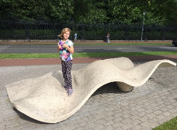
Marion Weeks on wavy sculpture

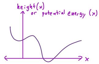
In introductory physics, we often draw a curvy hill and note that the potential energy is proportional to the height of that hill. A ball placed on the hill will roll down to the bottom, to minimize its potential energy. This is a simple "energy landscape" where the physical landscape is also the same shape as the energy landscape. When we draw this out, we draw a curve that's a function of one coordinate, x. 1D energy landscape
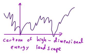
A fancier idea dates back to Marcelin in 1914 and Goldstein in 1969, that for a bunch of particles interacting with each other, the potential energy is a function of all of their coordinates. If we're talking about 100 particles in a three-dimensional world, the total number of (x,y,z) coordinates is 300. Thus this energy landscape is impossible to visualize. In practice, many people just draw a really wiggly sketch to stand in for this idea. wiggly line, but still 1D landscape

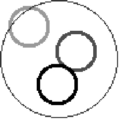
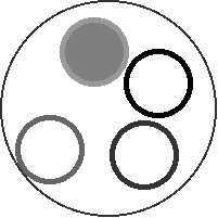
On the other hand, what about hard particles? These particles do not have any potential energy, so you can't think about an energy landscape in the same way. On the other hand, we can define an entropy landscape (or equivalently, a free energy landscape). And specifically, we came up with a simple model system for which we can do this exactly, the system shown in the animation at right. These are three hard particles that cannot overlap, diffusing in a circular container. Occasionally one of the disks passes through the middle of the other two. It's random which disk does that. Click this link, or the image at right, to see an animation of this system.

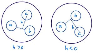
In this system there are two "equilibrium" states, shown in the image at right. One has the disks in order (abc) clockwise, and the other has the order (abc) counterclockwise. To describe the system, we'd need to specify the (x,y) coordinates of each of these disks: so, a total of six numbers. But, we can simplify this by defining the variable h as shown in the sketch. This is the height of disk c above the line defined by the disks a and b. This is defined as positive or negative depending on the orientation of the three disks. So, the sign of h tell us which state the system is in.

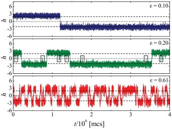
Thus, transitions of the system from one equilibrium configuration to another require h to change sign -- in other words, to pass through 0. This could be disk c going through the middle of disks a and b (see sketch at right), or also if one of the disks a or b passes through the middle of the other two, that also works. You can see the transitions in the graph below.


Sketch for h=0.
trajectories h as a function of time
Trajectories for h depending on the system size.
Which brings up an interesting point: the ease of making a transition relates to how easy it is to have the three disks align along the diameter of the system. The smaller the overall system size, the harder it is for the three disks to align. Thus the bottom red curve in the h(t) plot is for a larger system, and the top blue curve is for a smaller system. We like this aspect of our model system because it's a bit like glassy behavior: molecules in a glass rearrange less frequently as the glass gets cooled. Likewise, our disks rearrange less frequently as the system gets smaller.

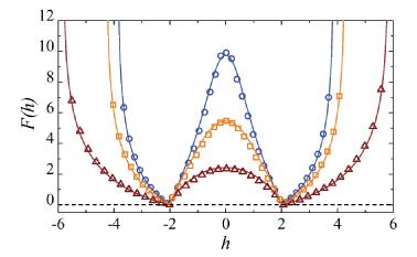
At this point, we're ready to make our landscape. We run the simulation for a very long time and count how many times we see each value of h; in statistical mechanics, that's called Omega(h). We take the logarithm of Omega(h) and that's the entropy S(h). The free energy is the negative of the entropy: and that is graphed at the right for three different system sizes. The low points at -2 and +2 correspond to the equilibrium states -- the most common values of h. The bump at h=0 is an entropy barrier, meaning that it is difficult to change from one equilibrium state to the other because h = 0 is a low entropy state. Specifically, the entropy barrier is largest for the smallest system size, which qualitatively matches the discussion of the trajectories above. In other words, the smaller the system, the harder it is to get a transition.

But the really fun point is that the graph at right is a real free energy landscape: not a sketch.

free energy landscape graph
All of the above work was published in the 2012 article by Hunter & Weeks (see the reference at the top of this page).
We then were curious how these results are modified for soft disks: disks that can overlap. In this case, temperature matters as well as the system size. Click here to see an animation of the soft disk system. We showed that for soft disks, you can still think about a free energy landscape. More significantly, we demonstrated that as the system becomes "glassy" (disk swapping becomes more rare), the free energy barriers had nontrivial contributions from both potential energy and entropy. This gives some insight into why glasses might be non-Arrhenius. That phrase just means that as glasses cool down, they don't just behave as if there is a simple potential energy barrier that gets harder to cross at lower temperatures. We're seeing the same phenomenon: at constant system size, our system has a constant potential energy barrier. But the slowing is more dramatic just crossing this barrier, and the additional effect is due to entropy. This was published in the 2016 article by Du & Weeks (see the references at the top of this page).

Next we came up with some ideas for free energy landscapes for four particles. Click here to see an animation of the four disk system. This work was published in the effect is due to entropy. This was published in the 2020 article by Weeks & Criddle (see the references at the top of this page). This article made three main points:
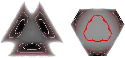
  • Multiple free-energy landscapes can be constructed to represent the same system. (The article gives three examples; they are pictured below. The Hunter & Weeks article also gives two examples for the three disk system.)
  • The nonlinear mapping used to create free energy landscapes can distort the free energy barrier height. (And this doesn't mean that any of the landscapes are "wrong.")
  • Diffusion rates on the free energy landscape can vary spatially. (Which relates to the free energy barrier height.)
two free energy landscape images
The red contours are spaced in 2 kT intervals. There are six equilibrium states, but these two free energy landscapes collapse the six states into three. The benefit is that the landscapes are two dimensional (which is a great reduction from the eight dimensional space needed to describe the original system). Below is an example trajectory of the system moving through the left landscape.
free energy landscape
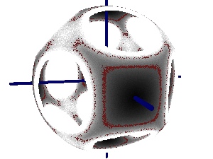
This free energy landscape is three dimensional. The equilibria are the faces of a cube (where the blue coordinate axes are located). Transitions between states require the system to pass through the corners of the cube, which are triangular in shape. What would be the edges of the cube are instead large circular holes, which indicate forbidden states -- places in the landscape that correspond to some of the four disks overlapping, which is forbidden in this model. Like the images at left, the red contours are spaced by 2kT.
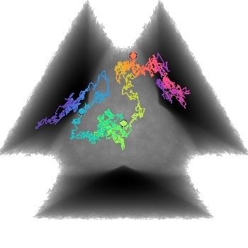
trajectory in free energy landscape The picture at left shows a trajectory through one free energy landscape. The system starts at the upper right (purple/red), goes through the orange to green to blue regions, and then ends at the left (blue/purple). This transition corresponds to the disks moving in real space such that two of them swap positions; see the Weeks & Criddle paper for more details.


Future/ongoing work: What do these landscapes look like for more than four disks? Clearly they will be higher dimensional and likely impossible to directly visualize; but perhaps we can take 2D or 3D cuts through a higher dimensional landscape and learn something useful. How might these ideas apply for a large number of particles? And, how might the landscapes look or differ for 3D situations? Everything described above is a model system, but the ultimate goal is to understand free energy landscapes for more realistic and interesting systems (in other words, large systems).


For more information, please contact Eric Weeks <weeks(at)physics.emory.edu>