poly_voronoi: Radical Voronoi & Delaunay

Program files (you need all three):

• poly_voronoi.pro
• radicalpoint.pro
• createperiodicboundary.pro

• And if you want to try the example out, download this data file: flat.txt (format: [x,y,radius])

• poly_voronoi.zip -- contains the three .pro files and 'flat.txt'

The regular Voronoi diagram considers a set of points in a plane, and then constructs polygons around each point. Each polygon is the region of the plane closer to the point within the polygon than to any other point. These polygons thus tile the plane. (The idea of Voronoi polygons idea generalizes to higher dimensions, for example, Voronoi polyhedra in 3D.)

The Delaunay triangulation is dual to the Voronoi diagram. For the Delaunay triangulation, any two points for which their Voronoi polygons share an edge are connected by a line in the triangulation. Those lines tile the plane with triangles. Sometimes this is used to identify nearest neighbor points: that is, any points connected in the Delaunay triangulation are neighbors. If you'd like to do Voronoi polygons or Delaunay triangulations, use IDL's built-in QHULL function, it will do it all for you.

The "radical" Voronoi / Delaunay idea is to include information about each point -- not all points are the same. For example, perhaps the points are actually the centers of circles of various sizes, so we wish to treat larger circles differently from smaller. Sometimes this is called a power diagram although I find that Wikipedia explanation a bit hard to follow. The examples below should be clear enough. In general, if you have a close packed set of circles of various sizes, then the radical Voronoi polygons will wrap nicely around each circle.

Let's see how this works.

IDL> a=readtext('flat.txt')
IDL> pv = poly_voronoi(a[0:1,*],a[2,*],ri,ob,tri,Box=[0,1,0,1])

IGL> ; next five lines:  draw the circles with their various radii
IDL> cx=cos(findgen(101)/100.*2.0*3.14159)
IDL> sx=sin(findgen(101)/100.*2.0*3.14159)
IDL> na=n_elements(a(0,*))
IDL> plot,a[0,*],a[1,*],/nodata,/iso
IDL> for i=0,na-1 do oplot,a(0,i)+cx*a[2,i],a(1,i)+sx*a[2,i],col=11680941,thick=2
IDL>
IDL> ; this next for-loop:  draw radical Voronoi polygons
IDL> for i=0,na-1 do begin & $
IDL>    ri0 = ri[i] & ri1 = ri[i+1] & $
IDL>    if (ri1 gt ri0) then begin & $
IDL>        idx = ri[ri[i]:ri[i+1]-1] & $
IDL>        idx = [idx,idx[0]] & $
IDL>        oplot,pv(0,idx),pv(1,idx),col=9234984 & $
IDL>     endif & $
IDL> endfor

Which generates this image:

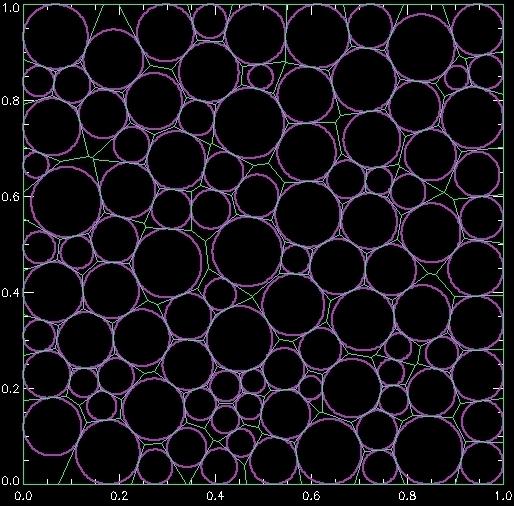
What's happening here? The variable ri contains "reverse indices" which work the same way as the HISTOGRAM IDL command works. The first na entries of this array are indices that point to later in the array. Those locations pointed at can be of arbitrary length, a big benefit of this array structure. The for-loop above grabs the starting and ending point from the first part of the array, where these points indicate where the data are stored in the second part of the array. What is stored in that second part is the indices of the Voronoi vertices that correspond to a specific Voronoi polygon around a specific particle in the original array, that is, one of the circles. So by grabbing those vertices and plotting them, we draw one polygon. The for-loop loops through all the possible polygons, which is one per particle.

In rare circumstances, something doesn't have a polygon: thus the "if" statement to check that we have at least one vertex. I'm not sure what causes those rare circumstances, I just know that adding this in was useful occasionally, and I didn't have the time to track down what was going wrong in those rare cases.

The ob variable returned by the program is 1 if a particle is on the edge, and 0 otherwise.

There is also an area keyword to return the Voronoi polygon areas.

We can also do the radical Delaunay triangulation:

ntri=n_elements(tri(0,*))
IDL> plot,a[0,*],a[1,*],/nodata,/iso
IDL> for i=0,na-1 do oplot,a(0,i)+cx*a[2,i],a(1,i)+sx*a[2,i],col=11680941,thick=2
IDL>
IDL> for i=0,ntri-1 do begin & $
IDL>     pts=[tri[0,i],tri[1,i],tri[2,i],tri[0,i]] & $
IDL>     if (max(pts) lt na) then $
IDL>         oplot,a[0,pts],a[1,pts],col=13808670 & $
IDL> endfor

which generates this image:

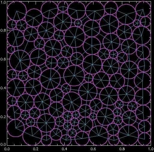
Here the tri array is simpler to understand: it's a 3 by N list of integers that correspond to trios of the original data points which are part of a triangle. Thus by connecting those (x,y) points, we draw the triangle, and by looping over all the triangles, we draw all of the connections.

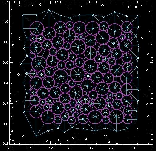
The poly_voronoi program deals with boundary conditions in a specific way, using the createperiodicboundary code. This program takes the original data and adds new data on all sides of the original data. For rigid boundaries, the new data is a reflected image around the boundary. For periodic boundaries, the new data is the periodic image of the original data. (You can see that despite the name which suggests periodic boundaries only, the program can also do rigid boundaries.) So when the Delaunay triangulation is calculated, it can connect points in the original data set to points in the image data. These points have indices higher than the total number of points in the original data. The IF statement above screens out drawing those connections. If you want to see those connections, it's best to just generate the data using the createperiodicboundary code:

IDL> x=a[0:1,*]
IDL> xp=createperiodicboundary(x,[0,1,0,1],['R','R'])
IDL> 
IDL> plot,xp[0,*],xp[1,*],/nodata,/iso,xr=[-0.2,1.2],yr=[-0.2,1.2],/xs,/ys
IDL> oplot,xp(0,*),xp(1,*),ps=4
IDL> for i=0,na-1 do oplot,a(0,i)+cx*a[2,i],a(1,i)+sx*a[2,i],col=11680941,thick=2
IDL> for i=0,ntri-1 do begin & $
IDL>     pts=[tri[0,i],tri[1,i],tri[2,i],tri[0,i]] & $
IDL>     oplot,xp[0,pts],xp[1,pts],col=13808670 & $
IDL> endfor

Here I'm drawing circles over the original data, but also showing points where the image data exist. Here's the result:

For createperiodicboundary, the first argument is the data. The second is the corners of the data (xmin,xmax,ymin,ymax). The third is the boundary condition: 'R' for rigid and 'P' for periodic. There is also an optional "DIM" keyword: "DIM=3" will work with 3D data, in which case you can also provide (zmin,zmax) and a boundary condition in Z.

I'll leave it as an exercise for the reader as to how to best deal with periodic boundary conditions. That is, if you just want a list of circles that are neighbors according to the radical Delaunay triangulation, and you have periodic boundary conditions, then you'll want to use the information about connections to the image particles as ways to connect the original particles on opposite sides of the periodic boundaries. I haven't needed to do this yet, so I have not yet worked out a solution to this problem. My guess is that you could use the particle index modulo the number of particles to quickly identify which original particle is the correct Delaunay neighbor. That is, if you have 100 particles and the triangulation array identifies neighbors (17,712,520) then I believe the correct neighbors of that Delaunay triangle are (17,12,20) -- but they are only neighbors by wrapping around the periodic boundaries.

Contact Eric:

• Eric Weeks: erweeks(at)emory.edu